Preamble
Tools: QGIS
Data: Sentinel-2 sample images (provided during the session)
Goal: understand how satellite images are structured and how to explore them using a GIS environment
Learning Objectives
By the end of this session, students will be able to:
Identify key properties of a satellite image (dimensions, spatial resolution, CRS, origin coordinates)
Explore raster characteristics (number of bands, data type, NoData values)
Configure the display of multispectral images (contrast, color composites, NoData handling)
Select appropriate band combinations to highlight land cover features
Interpret basic land cover types from satellite imagery
Course Material
Data and tools required for this lab session are available below 👇
📂 Labworks data:
Download the dataset containing the Sentinel-2 bands:
After downloading:
Unzip the archive
Place the extracted folder in a known location on your computer
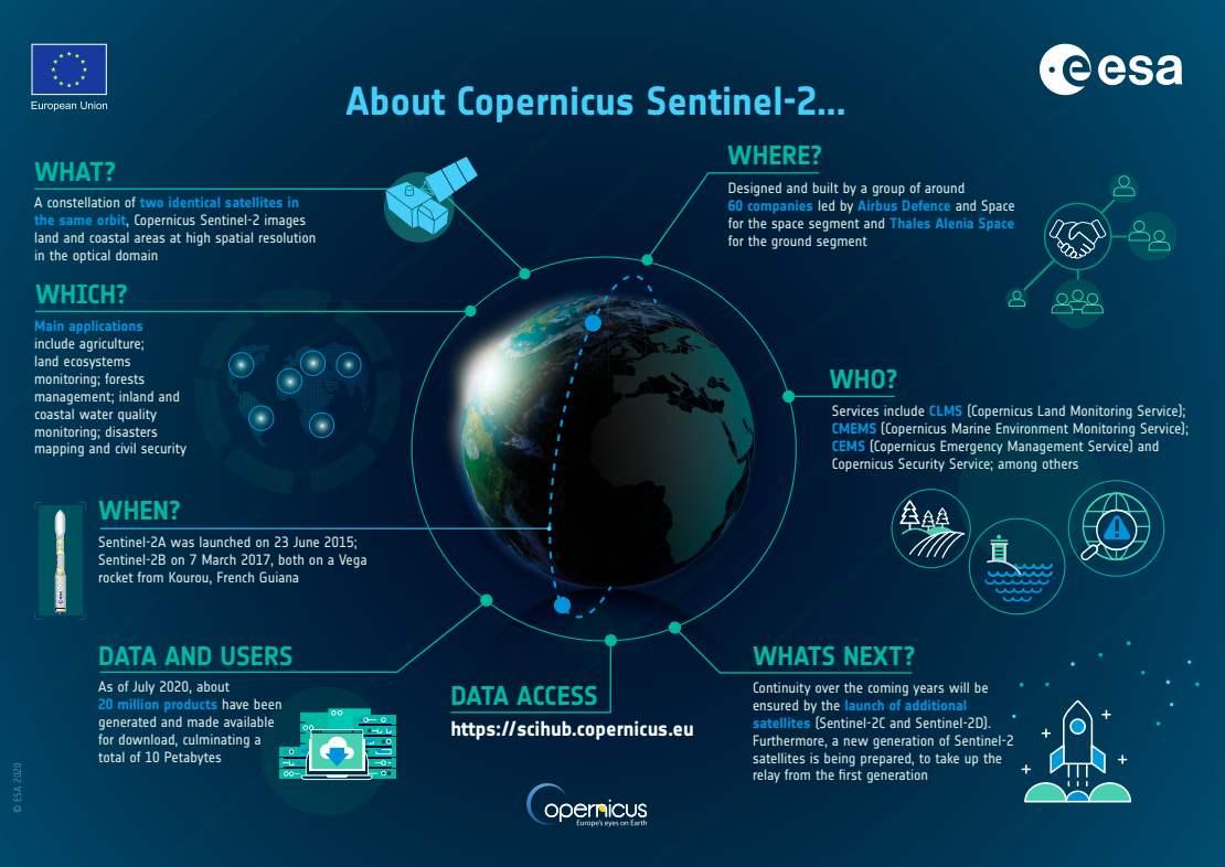
🛰️ The Sentinel-2 mission:
Sentinel-2 is part of the Copernicus Earth Observation programme of the European Union, developed and operated by the European Space Agency (ESA).
The mission consists of a constellation of satellites equipped with a Multispectral Instrument (MSI) designed to monitor land surfaces, vegetation, soils, water bodies and coastal areas. :contentReference[oaicite:0]{index=0}
Sentinel-2 provides high-resolution optical imagery with 13 spectral bands ranging from the visible to the shortwave infrared region of the electromagnetic spectrum. :contentReference[oaicite:1]{index=1}
These bands are acquired at three spatial resolutions:
| Spatial resolution | Number of bands |
|---|---|
| 10 m | 4 bands |
| 20 m | 6 bands |
| 60 m | 3 bands (mainly designed for atmospheric correction purposes) |
This combination of spectral richness, spatial resolution and frequent revisit time (~5 days) makes Sentinel-2 particularly well suited for applications such as:
vegetation monitoring
agriculture and crop mapping
land cover classification
disaster monitoring
environmental change detection
 Source: ESA Copernicus Sentinel-2 mission overview.
Sentinel-2 spectral bands
The Sentinel-2 sensor records reflectance in multiple regions of the electromagnetic spectrum, including:
Visible (VIS)
Near Infrared (NIR)
Shortwave Infrared (SWIR)
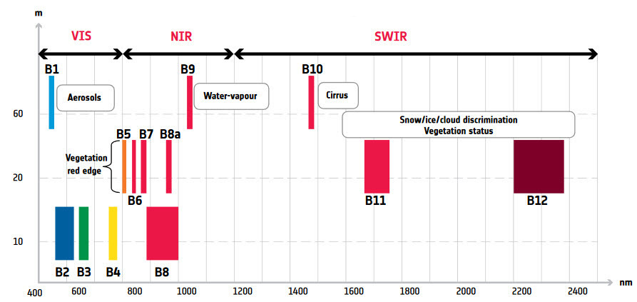
These spectral bands allow the analysis of different properties of the Earth’s surface, such as vegetation health, soil moisture, and water content.
🛠 Labworks tools:
If QGIS is not installed on your computer, you can download the LTR (Long Term Release) from the official website: https://qgis.org
For this session, a portable version of QGIS is also provided.
Steps to run QGIS portable:
Download the archive below
Unzip the folder
Launch QGIS by double-clicking on:
launch_qgis_portable.bat
📦 Portable QGIS: 📥 QGIS
Tasks
Task 1 – Data download
Download the dataset from the link provided above.
Unzip the archive.
Place the extracted folder in a known directory on your computer.
Inside the folder you should find several Sentinel-2 spectral bands stored as raster files.
Task 2 – Opening the data in QGIS
Open QGIS
Create a new project
Load the raster files
Menu: Layer → Add Layer → Add Raster Layer
Once loaded, the layers will appear in the Layers panel.
Questions
What type of data are these files?
How many raster layers are provided?
Task 3 – Inspecting image properties
In QGIS, explore the properties of the satellite image.
Step 1 – Raster properties
Right-click on one of the raster layers
Open Properties
Go to the Information tab and observe the different characteristics
Questions
What are the image dimensions (rows and columns)?
What is the pixel size?
Which CRS is used?
How many bands does the dataset contain?
What is the data type of the raster values?
Is a NoData value defined?
Step 2 – Pixel values
Use the Identify Feature tool in the QGIS toolbar 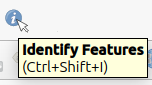 and click on different pixels corresponding to various land cover types:
water
vegetation
urban areas
forest
Questions
Do the pixel values differ between land cover types?
Which land cover types show the highest values in the NIR band?
Task 4 – Exploring individual spectral bands
Each band represents the reflectance of the Earth’s surface measured at a specific wavelength of the electromagnetic spectrum.
The Sentinel-2 dataset provided in this lab includes the following bands:
| Band | Description |
|---|---|
| B2 | Blue |
| B3 | Green |
| B4 | Red |
| B8 | Near Infrared (NIR) |
| B11 | Shortwave Infrared (SWIR) |
Questions
Which band highlights vegetation the most?
Which band makes water bodies appear darkest?
Task 5 – Creating a multiband stack (VRT)
The Sentinel-2 bands are provided as separate raster files, each corresponding to a different wavelength. To work with them together (for visualization or analysis), we first create a multiband stack. Instead of creating a new raster file on disk, we will create a Virtual Raster (VRT).
A VRT is a lightweight file that references existing rasters and virtually combines them into a single multiband dataset, without duplicating the data on disk.
Steps
Open the tool:
Raster → Miscellaneous → Build Virtual Raster (VRT)
Add the 5 spectral bands in the following order:
B2 B3 B4 B8 B11Check Place each input file into a separate band
Set Resolution → Highest resolution
Some Sentinel-2 bands have different spatial resolutions (10 m or 20 m). Choosing the highest resolution will resample the 20 m bands to 10 m so that all bands share the same grid.
For the resampling method, select:
Nearest neighbourSave the file in a known directory as:
S2_band_stack.vrtRun the tool.
The result is a multiband virtual raster that combines the five Sentinel-2 bands into a single layer.
Task 6 – Creating a Natural Colour Composite
Satellite images are often visualized by combining three bands.
To create a natural colour composite:
Right-click the VRT layer
Open Layer Properties
Go to Symbology
Select Multiband color
Assign the following bands:
| Channel | Band |
|---|---|
| Red | B4 |
| Green | B3 |
| Blue | B2 |
This combination approximates what the human eye sees.
Questions
Can you identify vegetation?
Can you identify water bodies?
Can you identify urban areas?
Task 7 – Creating a False Colour Composite
False colour composites highlight specific land surface features.
Use the following band combination:
| Channel | Band |
|---|---|
| Red | B8 |
| Green | B4 |
| Blue | B3 |
In this representation:
Vegetation appears bright red
Water appears dark
Urban areas appear grey or cyan
Questions
Why does vegetation appear bright in this composite?
Which areas correspond to dense vegetation?
Task 8 – Exploring Spatial Resolution
Zoom in on Band B2
Then zoom in on Band B11
Observe the differences in pixel size.
You can also consult the metadata to verify the spatial resolution.
Questions
What differences do you observe between the two bands?
Which band has the higher spatial resolution?
How does spatial resolution affect the level of detail in the image?
Task 9 – Interpreting land cover
Using the different visualizations, try to identify:
forest areas
agricultural fields
water bodies
urban areas
Using the identify features tool, record approximate pixel values for several land cover types in the following bands:
Blue (B2)
Red (B4)
Near Infrared (B8)
Questions
Do different land cover types show different value ranges?
Which band best separates vegetation from water?
Further Reading and Resources
Sentinel-2 band descriptions: https://
custom -scripts .sentinel -hub .com /custom -scripts /sentinel -2 /bands/ Sentinel-2 mission documentation: https://
www .esa .int /Applications /Observing _the _Earth /Copernicus /Sentinel-2 ESA Copernicus Programme: https://
www .esa .int /Applications /Observing _the _Earth /Copernicus /Introducing _Copernicus
Troubleshooting – QGIS portable version
Some students may experience issues where raster processing tools do not appear or do not work correctly in the portable version of QGIS.
If this happens, you can reload the core plugins manually using the Python console.
Steps
Open the Python Console in QGIS
Menu:Plugins → Python ConsolePaste and run the following code:
from qgis.utils import unloadPlugin, loadPlugin, startPlugin

core_plugins = ["processing", "db_manager", "MetaSearch", "grassprovider"]

for plugin in core_plugins:
    try:
        print(f"Reloading plugin: {plugin}")
        unloadPlugin(plugin)
        loadPlugin(plugin)
        startPlugin(plugin)
        print(f"{plugin} successfully reloaded\n")
    except Exception as e:
        print(f"Error while reloading {plugin}: {e}\n")

print("Done — plugins should now be active.")

This will reload the core processing plugins and usually fixes issues with the Raster Calculator or Processing tools.